
1 Trigonometric Ratios
Trigonometric functions extend the concept of trigonometric ratios. Trigonometric ratios relate the ratios of the sides of a right-angled triangle to its angles. As explained in Section 2, trigonometric functions are defined using the circle; however, the fundamental idea still relies on considering right-angled triangles in trigonometric ratios. Before learning trigonometric functions, it is useful to have a brief understanding of trigonometric ratios.
Trigonometric ratios relate the angles and side ratios of the right-angled triangle shown in Figure 1. Specifically, “\sin \theta represents the ratio of the side opposite to \theta to the hypotenuse,” “\cos \theta is the ratio of the side adjacent to \theta to the hypotenuse,” and “\tan \theta represents the ratio of the two legs other than the hypotenuse.”

2 Definition of Trigonometric Functions
Trigonometric functions are defined using the circle as shown in Figure 2.
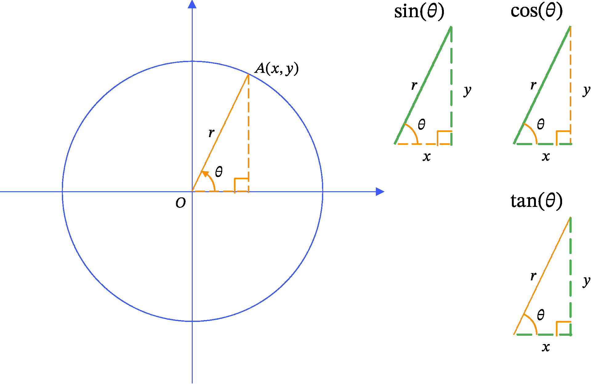
Consider a circle of radius r. Measure the angle \theta counterclockwise from the positive direction of the x-axis and plot the point A(x, y) on the circumference. Using the radius r and the coordinates x and y of point A, trigonometric functions are defined:
\begin{aligned} \sin \theta &= \frac{y}{r}\\ \cos \theta &= \frac{x}{r}\\ \tan \theta &= \frac{y}{x} \end{aligned}
3 Relationship Between Trigonometric Functions and Ratios
Comparing Figure 1 and Figure 2, one can see that the right-angled triangle used in defining trigonometric ratios fits inside the circle that defines the trigonometric functions. Indeed, for 0 < \theta < 90^\circ, there is no difference between the values expressed by trigonometric ratios and functions. However, trigonometric ratios fundamentally require the existence of a right-angled triangle. For example, at \theta = 0^\circ or \theta = 90^\circ, it is impossible to form a right-angled triangle, so trigonometric ratios cannot be defined.
Trigonometric functions extend the trigonometric ratio concept by not requiring a right-angled triangle. Instead, they use the radius of the circle and the coordinates of the point on its circumference. Under these conditions, they define the trigonometric concepts even for angles for which trigonometric ratios cannot be defined. This extension is what trigonometric functions represent.
4 Degrees and Radians
Trigonometric ratios often use angles with the unit “degree” (^\circ) such as 0^\circ or 45^\circ. This way of expressing angles is called the degree measure and is widely used in everyday life.
On the other hand, trigonometric functions express angles using the radian measure rather than degrees. The radian (unit: rad) is defined as the ratio of the length of an arc of a circle to the radius of that circle (Definition 1).
Definition 1 (Definition of an Angle Using Radians) \theta = \frac{l}{r}.
Here, l is the length of the arc, and r is the radius of the circle.
In Definition 1, given a circle with radius r, choose a point A(r, 0) and let point B on the circumference be reached by measuring an arc length l counterclockwise (Figure 3). The angle \theta determined in this way is uniquely defined by Definition 1. This angle is expressed in radians.

There is a relationship between degrees and radians expressed as follows:
360^\circ \Leftrightarrow 2 \pi \tag{1}
5 Trigonometric Functions Are Independent of the Radius
Although trigonometric functions are defined using a circle (Figure 2), their values do not depend on the radius of the circle. No matter what radius you choose, if the angle \theta remains the same, the trigonometric functions always have the same value.
This justifies that when calculating the values of trigonometric functions, you may consider a circle of any convenient radius to simplify computations (Section 6).
6 Calculating Trigonometric Functions
Using the definitions of trigonometric functions shown in Figure 2, you can calculate the special values of trigonometric functions. Let us calculate the values of trigonometric functions for \theta = \frac{\pi}{3}.
From Equation 1, we know that 2 \pi corresponds to 360^\circ. Since \frac{\pi}{3} equals \frac{1}{6} of 2 \pi, by analogy, \frac{\pi}{3} corresponds to 60^\circ.
It is well known that a right-angled triangle with an angle of 60^\circ has side ratios 1 : 2 : \sqrt{3}. Therefore, it is suitable to consider a right-angled triangle with a radius of 2 as in Figure 4. From Section 5, using a circle of radius 2 to calculate values of the right triangle is perfectly valid.

Following the definitions in (Figure 2), we calculate:
\begin{aligned} \sin \theta &= \frac{\sqrt{3}}{2},\\ \cos \theta &= \frac{\sqrt{1}}{2},\\ \tan \theta &= \frac{\sqrt{2}}{1} = 2. \end{aligned}
In this example, we use a circle of radius 2. For other angles such as \theta = \frac{\pi}{4}, it is easier to consider an isosceles right triangle and use a circle of radius \sqrt{2}.
7 Trigonometric Identities
There are many trigonometric identities, but most can be proved or derived easily by using definitions or addition formulas. Understanding the methods to prove these identities significantly reduces the number you need to memorise.
Rather than rote learning, comprehending and being able to prove the identities yourself deepens your understanding of trigonometric functions, enhances your ability to apply them, and leads to better long-term retention.
Trigonometric identities are classified into two groups based on their proof method: (1) those proved using the definition, and (2) those proved using addition formulas. I recommend understanding the identities based on this classification. For a comprehensive summary, please see the articles below:
Identities proved using the definition include basic trigonometric identities, negative angle trigonometric identities, complementary angle identities, and supplementary angle identities. Please check the following articles for the proofs of each identitiy:
- Proofs of basic trigonometric identities
- Proofs of negative angle identities
- Proofs of complementary angle identities
- Proofs of supplemetary angle identities
Along with the definition, it is advisable to memorise the addition theorems. To enhance your application skills with trigonometric functions, you should understand the proofs of the addition theorems. However, recalling these theorems through proof can be quite tiresome. Therefore, ensure you remember both the definition and the addition theorems.
8 Graphs of Trigonometric Functions
When studying functions, we often rely on their graphs. Exploring the graphs of trigonometric functions helps deepen your understanding of their properties.
8.1 Periodicity of Trigonometric Functions
As shown in Figure 5, the graphs of trigonometric functions exhibit a periodic pattern. Both y = \sin x and y = \cos x have a fundamental period of 2 \pi, whereas y = \tan x has a period of \pi. A period refers to the change in x that brings the function back to the same value. More precisely, a constant p is a period of the function f if:
f(x) = f(x + p)
This equation means that for any x in the domain, shifting by p results in the same y value. For example, in Figure 5 (a), at x = 0, y = 0, and at x = 2 \pi, which is 2 \pi shifted from 0, y also equals 0.
Although y = 0 also occurs at x = \pi, shifting x = \frac{\pi}{2} (the peak) by \pi leads to x = \frac{3 \pi}{2}, where the function value corresponds to a trough rather than the same y value. Therefore, \pi is not a period of y = \sin x.
Similarly, y = \cos x has period 2 \pi, showing oscillations similar to \sin x.
In contrast, y = \tan x has a period of \pi, and it is undefined at points like x = \frac{\pi}{2} or x = -\frac{\pi}{2}.

Purple bar: period. Yellow bar: amplitude.
8.2 Amplitude, Maximum and Minimum Values of Trigonometric Functions
“Amplitude” refers to the height of the wave from its central position to its peak. In figures Figure 5 (a) and (b), the yellow bar represents the amplitude. The centre of the wave height corresponds to the x-axis. Both y = \sin x and y = \cos x have an amplitude of 1.
As shown in Figure 5, the amplitude essentially equals the maximum value. Therefore, the maximum and minimum values of y = \sin x and y = \cos x are 1 and -1 respectively. On the other hand, y = \tan x takes any real value from - \infty to \infty.
8.3 Domain and Range of Trigonometric Functions
A function relates each input value to exactly one output value. The set of all possible input values is called the “domain,” and the set of all possible output values is called the “range.”
For trigonometric functions, the domain consists of all possible angles. As shown in Figure 5, we can consider the domain of y = \sin x and y = \cos x as all real numbers. In contrast, y = \tan x is not defined at x = \frac{\pi}{2} + n \pi, where n is any integer. Here, \mathbb{Z} represents the set of all integers (Table 1).
Since y = \sin x and y = \cos x take values between -1 and 1, their range is -1 \le y \le 1. Meanwhile, y = \tan x can take any real number, so its range is -\infty < y < \infty (Table 1).
| Function | Domain | Range |
|---|---|---|
| y = \sin x | -\infty < x < \infty | -1 \le y \le 1 |
| y = \cos x | -\infty < x < \infty | -1 \le y \le 1 |
| y = \tan x | All real numbers except x = \frac{\pi}{2} + n\pi, n \in \mathbb{Z} | -\infty < y < \infty |
8.4 Even and Odd Functions in Trigonometry
A notable feature of trigonometric functions, y = \sin x, y = \cos x, y = \tan x, is that they are even or odd functions. Simply put, these functions satisfy the following conditions:
- Even function: The graph is symmetrical about the y-axis.
- Odd function: The graph is symmetrical about the origin.
As shown in Figure 5, the graph of y = \sin x is symmetric about the origin (rotating it 180^\circ around the origin results in the same graph), so it is an odd function. Similarly, y = \tan x is also an odd function. Meanwhile, y = \cos x is symmetric about the y-axis (folding along the y-axis matches the graph onto itself), so it is an even function.
9 Parallel Translation, Stretching and Shrinking of Trigonometric Graphs
Using the graphs shown in Figure 5 as a basis, we sometimes consider graphs that have been translated (shifted) or stretched/shrunk.
9.1 Parallel Translation of Trigonometric Graphs
Generally, the graph of a function y = f(x) translated by p units in the x-direction and q units in the y-direction is expressed as:
y - q = f(x - p).
This function is obtained by replacing x by x - p and y by y - q in y = f(x).
Therefore, the functions representing the graphs of these trigonometric functions translated by p horizontally and q vertically are:
\begin{aligned} y &= \sin x \quad \rightarrow \quad y - q = \sin (x - p), \\ y &= \cos x \quad \rightarrow \quad y - q = \cos (x - p), \\ y &= \tan x \quad \rightarrow \quad y - q = \tan (x - p). \end{aligned} \tag{2}
In Figure 6, examples of such translated graphs are shown. The purple dashed lines represent the original graphs, such as y = \sin x, while the translated graphs are shown with blue solid lines.
For example, in Figure 6 (a), the graph of y = \sin x is translated to y = \sin \left( x - \frac{\pi}{2} \right). Notice the purple dot on the dashed line graph moves to the blue dot on the solid line graph.
Comparing with Equation 2, this example shifts the graph of y = \sin x by \frac{\pi}{2} along the x-axis.
In Figure 6 (c), the graph of y = \tan x is translated by \frac{\pi}{2} horizontally and by 1 vertically.

Parallel translation and scaling of trigonometric Functions
9.2 Scaling of Trigonometric Graphs
You can scale the graph of a trigonometric function along the y-axis or the x-axis. For example, the following equation represents scaling the graph of y = \cos x by a factor of a along the y-axis:
y = a \cos x. \tag{3}
In figure Figure 6 (b), the graph of y = \cos x is scaled by a factor of 2 along the y-axis.
On the other hand, the following equation scales the graph of y = \cos x along the x-axis by a factor of \frac{1}{b}:
y = \cos (bx). \tag{4}
This means that when b=2, as in y = \cos (2x), the graph is compressed to half its width along the x-axis. As a result, the number of wave peaks between -2 \pi \le x \le 2 \pi increases (see figure Figure 6 (b)).
9.3 Summary of Parallel Translation and Scaling of Trigonometric Graphs
Combining equations Equation 2, Equation 3, and Equation 4, the following equation expresses all these transformations of trigonometric graphs—parallel translation, scaling, or both—(shown here for y = \cos x, but the same applies to other functions):
\begin{aligned} y - q &= a \cos (b(x - p))\\ &\Leftrightarrow\\ y &= a \cos (b(x - p)) + q. \end{aligned}
The graph drawn b y this function has the following characteristics:
- Amplitude: \vert a \vert
- Period: \frac{2 \pi}{\vert b \vert}
- Horizontal (phase) shift: p
- Vertical shift: q
In figure Figure 7, the graph of y = 2 \cos \left(\frac{1}{2} \left(x - \frac{\pi}{2} \right)\right) + 1 is plotted. I encourage you to verify the amplitude, period, and both x-axis and y-axis shifts using this example.
![]()
The purple dashed line represents y = \cos x. The blue solid line shows y = 2 \cos \left(\frac{1}{2} \left(x - \frac{\pi}{2} \right)\right) + 1. The purple dots on the dashed line move to the dots on the solid line.
10 Conclusion
In this article, we have broadly covered the fundamental concepts of trigonometric functions. You can access more detailed explanations through the links provided within the text. Understanding the proofs of the formulas for trigonometric functions significantly reduces what you need to memorise. Use what you have learned here as a foundation to deepen your understanding of trigonometric functions further.


